
Autor: Marta Wysocka1,2, Michał Zeńczak1, Anna Czerwoniec1,2
1. VitaInSilica Sp. z o. o., ul. Krzemowa 1, Złotniki, 62-002 Suchy Las
2. Uniwersytet im. Adama Mickiewicza w Poznaniu, Wydział Biologii, ul. Umultowska 89, 61-614 Poznań
1. ChIP-seq EXPERIMENT
A lot of cellular functions strongly depend on protein-DNA interactions for instance: DNA-replication, recombination, gene expression, cell differentiation, cell cycle progression, chromosome stability and epigenetic silencing. Also chromatin is a combination of DNA and protein interactions. The proteins involved in maintaining the chromatin structure are called histones, including histone H1, 2A, 2B, 3 and 4. Histones bind to the DNA, package it tightly, change its structure to fit into the nucleus. Wrapped DNA carries the genetic information. Chromatin-coordinated genes control a variety of phenotypic changes in normal and diseased cells.
The DNA-protein interactions, according to their critical influence on cells, have been widely studied using multiple biochemical and genomic approaches. In vitro methods such as electrophoresis gel mobility shift (EMSA) and DNase I footprinting assays were very limited and that led to the development of new methods for analysing DNA-protein interactions. The most popular are ChIP, ChIP-chip and ChIP-seq. These techniques are useful in identifying regions of a genome associated with specific proteins within their native chromatin context. [1]
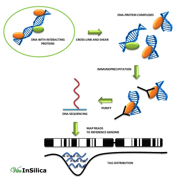
1.1 Chromatin Immunoprecipitation (ChIP)
ChIP is an effective method for identifying binding sites between the genome and the proteome. Mentioned technique consists of observation transcription regulation through histone modification or transcription factor-DNA binding interactions. ChIP is so popular and useful due to its ability for detection specific protein-DNA interactions which appear in cells. [2]
In addition, ChIP can be used with other techniques such as real time PCR, Southern and Western blot analysis. However, in PCR, knowledge of the target genes is essential to plan promoter-specific primers or probes. That is the reason why scientists decided to link a ChIP assay with genomic micro-array techniques (ChIP-chip), sequencing technology (ChIP-seq), or cloning strategies. This new approach led to the discovery of unknown gene sequences which can interact with proteins. ChIP-Chip and ChIP-seq methods provide a more global approach than ChIP assay. [1]
2. DATA ANALYSIS WORKFLOW
The output of a ChIP-seq assay contains short nucleotide sequences which probably are the binding sites of a given protein.[3] The main analytical steps of ChIP-seq data analysis workflow are: quality control, mapping, peak detection, motif analysis, annotation, and visualization.
In the first quality control step filtering out reads with poor quality bases, adaptors or other contaminants is done. Next, mapping to a reference genome is performed using programs such as Bowtie, BWA, MAQ or SOAP. As the second quality control step, only uniquely mapped reads are kept, the rest is filtered out to avoid potential PCR or optical duplicates.
A good quality human library is expected to have at least 70% of uniquely mapped reads. After achieving a high quality experiment, clustering of mapped reads around genomic locations is done. The most challenging step in the analysis workflow is the peak finding. Identification of clusters of enriched regions or differential binding of a protein between two or more biological conditions are the two main goals of peak detection algorithms [1][4]. In the last step, a motif analysis program such as MEME-ChIP or peak-motifs are used to assemble and evaluate regions found during the peak detection for motif discovery. That gives the opportunity to discover new binding motifs and also to verify already known motifs.[1] Alignment results can be visualized using UCSC genome browser as ChIP-seq signal coverage tracks. This allows for interpretation of peaks in the context of functionally relevant genomic regions. [1]
2.1. Mapping genome
Mapping of the sequenced DNA to a reference genome is one of the most crucial steps in the analysis as it identifies the genomic locations of bound DNA-binding enzymes, modified histones, chaperones, nucleosomes, and transcription factors (TFs). Hence showing the influence of these protein-DNA interactions on gene expression and other cellular processes. [5]
The most important data to consider after mapping is the percentage of uniquely mapped reads which varies between species. For human or mouse 70% is a normal score, whereas a result less than 50% is alarming. That lowered level can be caused by various reasons (e.g. excessive amplification in the PCR step, wrong read length, or problems with the sequencing platform). Sometimes obtaining a low percentage of uniquely mapped reads is unavoidable and if that’s the case, running a pair-end sequencing is recommended. Choosing the right number of mismatches to be allowed per read is also important. Read mappers allow users to specify that parameter and it has to be appropriate with the NGS platform of choice. This parameter can be obtained from the manufacturer. [5]
Defining the signal-to-noise ratio (SNR) is the next step in the ChIP-seq data analysis. This can be easily done via quality metrics such as strand cross-correlation (a built-in feature in some peak callers e.g. SPP or MACS) or IP enrichment estimation which is available in the software package CHANCE. Proceeding these measures makes possible to detect failure modes of ChIP-seq: insufficient enrichment by immunoprecipitation step, poor fragment-size selection, or insufficient sequencing depth. [5]
2.2. Peak detection
Peak detection is divided into four main parts: creating a profile, selecting candidate sites, calculating significance (p-value), determining cut-off threshold (i.e. false discovery rate – FDR); and normalization (not fully exploited). [4] Selection the peak detection algorithm and normalization method are core elements in the way to get meaningful interpretation of ChIP-seq data. Commonly used peak detection algorithms are MACS and SPP. [1] In present peak callers differences can be found in terms of signal smoothing and background modeling.
2.2.1. Creating a profile
The goal of this step is to obtain a ChIP profile by smoothing the tag counts, using or not correction tag-shifting effects. This improves summit resolution in a poor quality regions of experiment. A window with a pre-determined size, scans the genome and replaces the tag counts with its summed value (inside the window) at each site. That creates the profile. Software tools are capable of creating profiles in different ways. SPP and CisGenome marge consecutive windows above a threshold value. PeakSeq use non-overlapping windows and gather values from surrounding windows. Software which uses tag-shifting before the window sliding is MACs. F-seq and QuEST use the kernel density. F-seq substitutes the tag count for kernel density estimation and QuEST develops the strand-specific profile using mentioned value. [4] Several peak callers use alternative algorithm based on the shape of a peak (PeakSplitter, GPS). [5]
2.2.2. Selecting candidate sites or calling peaks
In the generated profile each unit with certain features is a candidate for a peak. Profile unit must have an absolute ChIP signal or enrichment in comparison to the background. The selected candidates are used to assess a fragment size and a distance of a tag shift. Regions that are not overlapping with peaks are useful to assess the parameters of the negative control. [4]
There are three types of ChIPed protein which determines the algorithm of peak callers. The first one is punctate-source transcription factors.They are the most frequent type of ChIP-seq data. That is why the majority of peak callers are designed for analysing these factors. For point-source factors it is recommended to analyze the shape of the peaks in order to reduce the final peak list using the R packages – polyaPeak and NarrowPeaks. [5]
The second type are proteins connected with epigenetic regulation (e.g. epigenetic marks – histone modification). Most of histone marks give a wider and weaker signal. That was the reason for designing new peak callers which could predict much broader regions from ChIP-seq data (SICER, CCAT, ZINBA, and RSEG). Some of the peak callers can use the option to increase “bandwidth” or to relax the “peak cutoff” e.g. SPP, MACS v.2 and PeakRanger. Combining multiple levels of enrichment is an approach used by e.g. MACS (version 2) and Scripture peak callers. [5]
The third type of ChIP-seq data gives mixed signals. Such data should be treated on the one hand as a point-source factor and on the other as factors with broad marks. There are few tools capable of analysing both narrow and broad peak calls – SPP, MACS, ZINBA and PeakRanger. However, with the correct set of parameters any algorithm for broad peak detection would work for this type of data. [5]
2.2.3. Calculating the significance of peaks
The next step is to remove noise from the control sample or other features of the genome sequence by using a specific background models. [5] There are different types of background models defining the significance of each peak. The Poisson distribution is used when the uniform effect of the negative control over the genome is assumed. When that is not the case – an alternative model is binomial distribution. [4] Many callers use different models for the statistical estimation of enriched regions: Poisson – CSAR, local Poisson – MACS, negative binomial – CisGenome, and zero-inflated negative binomial – ZINMA. More specialized callers such as HPeak and BayesPeak use the Hidden Markov Model. [5]
2.2.4. Determining cut-off threshold
Selecting a threshold value is a great challenge. When p-values from the relevant distribution are available it is possible to calculate an FDR. The other way to rank the peaks is usage of the peaks height or fold enrichment. Mentioned methods are used in tools which calculate the FDR as a ratio of the number of peaks called in the control to the number of peaks called in the ChIP data. In the post-processing step tag-shifting effects are considered and the fragment size of the library is predicted. Software tools perform that step in different ways. SPP estimate a tag shift by calculating the autocorrelation between positive- and negative-stranded tag counts. CisGenome improves effects of SPP in the two-step analysis. PeakSeq has no automatic option of tag shift correction, but allows user to set the fragment lengths. There are also some specialized tools developed towards analyzing ChIP peak types exploiting a hidden Markov model and clustering algorithm in order to find meaningful patterns [4].
2.2.5. Normalization
The are two types of normalization methods – linear and non-linear. Sequencing depth normalization is the most frequently used linear technique, which makes the numbers of reads in two different samples the same by multiplying the number of reads by a scale factor. A variant of the above-mentioned method is used in PeakSeq. CisGenome, MACS, and USeq which use a normalization factor, focusing on normalization against control samples. Scaling is also used in RPKM (Reads per Kilobase of sequence range per Million mapped reads) normalization method.
One of non-linear methods assume that changeable biological conditions do not impact on the global binding changes, called – Locally weighted regression with respect to mean and variance. The similar version of that non-linear normalization is implemented as MAnorm and also in the R package POLYPHEMUS. [5]
2.3. Assessment of reproducibility
The experimental results should be reproducible. To ensure that it is recommended to redo each of ChIP-seq experiment at least two times and in both cases verifying the reproducibility of reads and identified peaks. It is possible to measure the reproducibility of the reads by computing the Pearson correlation coefficient (PCC) of the reads counts at each genomic position. The value of PCC is between 0.3-0.4 for unrelated samples and 0.9 for samples in high-quality experiments. To get meaningful results of PCC it is important to remove the regions with high ChIP signals (e.g. regions near centromeres, telomeres, satellite repeats) before doing the analysis. At the level of peak calling Irreproducible discovery rate (IDR) analysis can measure the reproducibility. IDR quantifies the transition from real signal to noise by dividing peaks into a reproducible group and an irreproducible ones. This analysis return the number of peaks which are within the reproducibility threshold specified by user. According to reproducibility the number of peaks is more comparable across experiments after using a reproducibility based metric. [5]
2.4. Annotation
The annotation step is responsible for combining the ChIP-seq peaks with functionally relevant genomic regions (e.g. transcription start sites). The procedure starts with uploading the peaks and reads to a genome browser, which examines the regions in order to find associations with annotated genomic features. Systematic analysis performed by tools in packages like BEDTools describes genes with or without computing the distance from peaks to their nearest landmark. The result of mentioned analyses can be obtain by CEAS or the Bioconductor package ChIPpeakAnno. Then it can be compared with expression data (e.g. to check if a distance between gene and peak is connected with its expression) or gene ontology analysis which can be done using DAVID, GREAT or GSEA. (e.g. gene ontology analysis determine if the ChIPed protein is involved in particular biological processes). [5]
2.5. Motif analysis
There are few reasons to perform the motif analysis. The first is obvious and that is identifying the DNA-binding motif of transcription factors. What is more, it can identify the DNA-binding motif of proteins that bind in complex or in conjunction with the ChIPed protein, showing the mechanism of transcriptional regulation. That procedure is also useful to discover unanticipated sequence signals associated with histone modifications. In addition, when the motif of the ChIPed protein was known earlier, that analysis can be a base to assume about the success of the performed experiment. [5]
2.5.1. Steps in motif analysis
Motif analysis algorithms works on the genomic regions found by peak-callers. Firstly created is a set of sequences in FASTA format including all the meaningful ChIP-seq peaks. The next step is motif discovery. Only complementarity of strengths and weaknesses of algorithms provides to meaningful results so it is recommended to use two or more algorithms for one sequence set. Some of those algorithms are able to perform several motif analysis steps (MEME-ChIP, peak-motifs). Possibilities of software tools are described later. The next step is using motif comparison software to compare motifs from previous step with already known DNA motifs. That validates the presence of the ChIPed TF motif (or its TF-family) if its binding motif is known and also shows information about other TFs bounded near to the ChIPed TF. Afterwards information if other known DNA motifs are clustered near the centers of the ChIP-seq peaks gives central motif enrichment analysis. Performing the local version of that analysis is useful on regions centered on genomic landmarks. A motif spacing analysis is able to perform by limited number of software tools (SpaMo) and detects physical interactions between TFs. The last step, motif prediction maps and visualizes the genomic locations of the motifs, use a genome browser which allows to visualize matches between found motifs and the ChIPseq peak regions. [5]
2.5.2. Software tools and its comparison
Information given in the tool manual is specific and that can be the key to divide each tool into categories. First category: obtaining sequences, tools like Galaxy, RSAT, or UCSC Genome can be used. The second category includes tools for motif discovery (e.g. ChIPMunk, CisGenome, CompleteMOTIFS, MEME-ChIP, peak-motifs, Cistrome). To the third category belongs STAMP and TOMTOM frequently used in case of motif comparison. The fourth category consists of tools which provide information about motif enrichment/spacing – CentriMo and SpaMo. The last – FIMO and PATSER belongs to category of motif prediction/mapping. Except CisGenome every of mentioned tools have Web Servers. To obtain peak regions allows only Galaxy, RSAT, UCSC GB and Cistrome. Every software from second category can perform motif discovery. Motif comparison can be done by tools from Motif comparison and also CisGenome, CompleteMOTIFS, MEME-ChIP and peak-motifs. To central motif enrichment analysis are used MEME-ChIP, Cistrome and CentriMo, and local version of that analysis can performed by Cistrome and CentriMo. Motif spacing is only available by SpaMo. Motif prediction/mapping can be done by peak-motifs, Cistrome, FIMO and PASTER. [5]
3. ChIP-seq ABILITIES
Performing the ChIP-seq gives ability to pull out information about protein-DNA interactions, transcription factor binding locations or core transcriptional machinery, epigenetics, chromatin states or DNA methylation. [6]
3.1. Usage of ChIP-seq
Researches inter alia of Robertson G, Cheung’s and Reinke’s groups proves that ChIP-seq has its role in the discovery of transcription factor binding sites and network. Robertson et al. found supposed STAT1-binding regions in interferon γ-stimulated cells (41,582) and unstimulated (11,004). Also found 71% of loci known to contain STAT1 interferon-responsive binding sites. Results of Cheung’s group have shown that the AR transcriptional network obtained with ChIP-seq is ground-breaking to the strategic manipulation of AR activity for the removal process aimed at prostate cancer cells. Reinke used ChIP-seq to find the genome-wide binding sites of 22 transcription factors at various development stages in Caenorhabditis elegans. Results provide to determine features of transcriptional networks that regulate growing process of C. elegans. [1]
In addition different mechanisms involved in differential gene regulation can also be determine by using ChIP-seq. Mundadea at al. used ChIP-seq in researches of lysine mutations (K218/221 and K37). Theirs publication showed that in different physiological or disease states cells may use discovered mechanism to differentially regulate NF-kB-dependent genes. What is more experiments run by Paakinaho V group with usage of ChIP-seq showed that regulation of the glucocorticoid receptor (GR) activity in a target locus selective fashion that controls GR-dependent genes by SUMOylation is very complicated and has an impact on cell growth. [1]
Furthermore ChIP-seq is useful in the discovery of histone marks. Mikkelsen et al. use it assay to examine changes in chromatin stages due to maturation of the cell. Finding the role of tri-methylation (me3) on H3K4 and H3K2. Not only histone methylation is interesting as a histone mark in annotating the status of the gene transcription, also histone acetylation. That process examined Park et al. in a genome-wide analysis of H4K5 acetylation (H4K5ac) status. Inter alia they suggest that increase of the H4K5ac at consensus transcription factor binding sites (TFBS) in the promoter and proximal to the transcription start site (TSS) gives the gene the state of active transcription. Another histone modification determined as a mark of active gene transcription is histone phosphorylation, that has been studied by Tiwari group. They ran genome-wide ChIP-seq analysis to show the link between c-Jun NH2-terminal kinase (JNK), histone H3 Ser10 (H3S10) and promoters of a novel class of target genes which are noteworthy during stem cell differentiation into neuron. One more example in the discovery of histone marks is analysis of the epigenetic status of telomeres in Arabidopsis done by Vaquero-Sedas’s group. They used ChIP-seq data and discovered that short nucleosomal organization of telomeres reflects their higher destiny of histone H3 than that of centromeres. Moreover these experiment confirmed some theories about telomeres (e.g. telomeres have lower levels of heterochromatic marks than centromeres). [1]
3.2. Advantages of ChIP-seq over ChIP-chip
ChIP-seq method is the most popular ChIP variation. The biggest advantage of this method is the ability to decode millions of DNA fragments in a short time with a high efficiency and with a relatively low cost. [1]
First of all ChIP-seq does not require a predefined sequences of target genes. In comparison to ChIP-chip, ChIP-seq shows more. The second one is that the ChIP-seq allows to cover the most of repeated elements which are masked out in ChIP-chip method. Moreover the amount of DNA which is required for a successful ChIP-seq experiment is much more smaller than in ChIP-chip – about 10-50ng then in the older one – few micrograms. Another advantage of ChIP-seq in comparison to ChIP-chip is that multiplexing is possible. [6]Furthermore the information provided by ChIP-seq is more specific and quantitative than ChIP-Chip.[1] Relatively high resolution, low noise, and high genomic coverage are provided in ChIP-seq assay by using NGS, what cannot be guarantee during performance ChIP-chip experiment. [5]
REFERENCES
[1] RasikaMundadea, HaticeGulcinOzerb, Han Weia, Lakshmi Prabhua& Tao Luacd, Role of ChIP-seq in the discovery of transcription factor binding sites,differential gene regulation mechanism, epigenetic marks and beyond, Published online: 30 Oct 2014.
[2] Thermo Scientific Pierce, Protein Interaction Technical Handbook, Version 2, 57-59
[3] Krzysztof Chojnowski, Krzysztof Goryca, Tymon Rubel and Michal Mikula, jChIP: a graphical environment for exploratoryChIP-Seq data analysis, 26 September 2014
[4] Hyunmin Kim, Jihye Kim, Heather Selby, Dexiang Gao, Tiejun Tong, Tzu Lip Phang and AikChoon Tan, A short survey of computational analysis methods in analysingChIP-seq data, HUMAN GENOMICS. Vol 5. No 2. 117–123
[5] Timothy Bailey1, Pawel Krajewski, IstvanLadunga, Celine Lefebvre, Qunhua Li, Tao Liu, Pedro Madrigal, CennyTaslim, Jie Zhang, Practical Guidelines for the Comprehensive Analysis of ChIP-seq Data, PLOS Computational Biology, Vol 9. Issue 11, 14 November 2013
[6] http://medias01-web.embl.de/Mediasite/Play/94ec103b215c4b45a397400fde4029421d